\newcommand{\ra}{\rightarrow} \newcommand{\la}{\leftarrow} \newcommand{\Ra}{\Rightarrow} \newcommand{\La}{\Leftarrow} \newcommand{\Prob}[1]{\text{Pr}\!\left[#1\right]} \newcommand{\prob}[1]{\text{Pr}[#1]} \newcommand{\Expect}[1]{\text{E}\!\left[#1\right]} \newcommand{\expect}[1]{\text{E}[#1]} \renewcommand{\geq}{\geqslant} \renewcommand{\ge}{\geqslant} \renewcommand{\leq}{\leqslant} \renewcommand{\le}{\leqslant}

Randomized Algorithms

Peter Robinson

peter.robinson@mcmaster.ca
Navigation: Swipe or press space to advance.
Controls: Press f for fullscreen, m for table of contents, ESC for overview, '?' shows full list of shortcuts.

Why Randomized Algorithms?

  • Randomness is powerful resource for developing efficient algorithms with provable performance guarantees.
  • Compared to deterministic algorithms, randomized algorithms are often...
    • faster (or use less memory),
    • simpler to understand, and...
    • easier to implement, e.g. fewer special cases to worry about.
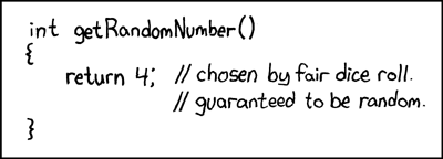
  • Important to understand foundations!

What this Course is about

  • How to use randomization to design better algorithms.
  • Discuss many applications where access to randomness provides significant benefits.
  • Equip you with necessary tools & techniques to analyze algorithms and also other random processes.
  • Provide you with a foundation for using probabilistic concepts in your own work.

Topics (tentative)

  • Concentration bounds
  • Probabilistic data structures
  • Fast graph algorithms
  • Verification using fingerprinting techniques
  • Random walks, Markov chains
  • The probabilistic method
  • Resilience against adversarial attacks in networks
  • Symmetry breaking in networks
  • Low-memory algorithms; dealing with dynamically-changing data

Marking Scheme (tentative *)

  • Homework assignments (40%)
  • Presentations of a research or survey paper (20%)
  • Reviews of peers' presentations (5%)
  • Final project (35%): choice of systems-focused or theory-focused

Prerequisites

  • Knowledge of data structures & algorithms (undergrad level) is recommended... but most parts of the course are self-contained
  • Undergrad-level discrete mathematics: discrete probability, basic knowledge of graph theory and combinatorics (e.g., how many ways can we choose an object such that...?)
  • Basics of the Big-O notation (e.g., being able to figure out the meaning of O(n \log n) , \Omega(n) , etc.)
  • Being able to write simple programs in <insert your programming language of choice here>
  • Unsure if this course is suitable for you? Come talk to me.

Resources

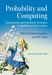
  • Material is loosely based on: Probability and computing: Randomized algorithms and probabilistic analysis by Michael Mitzenmacher and Eli Upfal. 2nd edition, 2017. Cambridge University Press. (Not required but recommended.)
  • Various resources on the web; to be added as we need them.
What are Randomized Algorithms?

Possible interpretations...

(1) Algorithms that make random choices during their executions. Use random number generator to decide next step.

(2) Algorithms that execute deterministically on randomly selected inputs.

Which interpretation is standard?

[Click to see answer.]
The answer is (1). Option (2) refers to average case analysis of algorithms.

Roadmap for Today

  • Verification of Matrix Multiplication
  • Fast Min-Cut Computation
  • Some techniques & tools along the way

Probability Space & Probability Axioms

Definition: A probability space (\mathcal{S},\mathcal{F},\text{Pr}) consists of...
  • a sample space \mathcal{S} : set of all possible outcomes
  • the set of events \mathcal{F} \subseteq 2^{\mathcal{S}} ; for discrete prob. space \mathcal{F}=2^{\mathcal{S}} .
  • the probability function \text{Pr} : \mathcal{F} \ra \mathbb{R}
Definition: A probability function \text{Pr} satisfies
  1. \forall E \in \mathcal{F}: 0 \le \Prob{E} \le 1
  2. \Prob{\mathcal{S}} = 1
  3. for all finite or countably infinite sequences of mutually disjoint events E_1,E_2,\dots , it holds that \Prob{\bigcup_{i\ge1}E_i } = \sum_{i\ge 1} \Prob{E_i} .
In discrete probability spaces: \mathcal{S} either finite or countably infinite.

The RAM model

We analyze time complexity in the Random Access Machine model.

  • Single processor, sequential execution
  • Each simple operation takes 1 time step.
  • Loops and subroutines are not simple operations.
  • Each memory access takes one time step, and there is no shortage of memory.

Application: Verifying Matrix Multiplication

The Problem

    Input: Given three n\times n matrices A , B , and C ; entries are rational numbers.

    Goal: Algorithm that verifies whether A \cdot B = C ; answers either "yes" or "no"

First Attempt: "Verification by Computation"
Compute (A \cdot B) and compare result with C .
Problem: standard matrix multiplication algorithm requires O(n^3) time. More sophisticated algorithms still take O(n^{2.3728639}) .
Can we solve this in O(n^2) time if we avoid computing A\cdot B ?

Tool: Sampling Uniformly at Random

Consider a finite set U of size m . We say that variable X is sampled uniformly at random (u.a.r.) from U when X is assigned to an element U , and each element in U has probability \frac{1}{m} to be the chosen one.
Example - "Sampling a random bit":
U = \{0,1\} . Variable X contains either 0 or 1 with equal probability.
Sampling 1 bit takes 1 unit of time in RAM model.

Algorithm for Verifying Matrix Multiplication

  • Steps:
  1. Sample n bits u.a.r. and store them in vector \vec{r} .
  2. Compute \vec{x} := B \cdot \vec{r} .
  3. Compute \vec{y} := A \cdot \vec{x} , so \vec{y} = A B \vec{r} .
  4. Compute \vec{z} := C \cdot \vec{r}
  5. if \vec{y}=\vec{z} then output yes, else output no.
  • Time:
  • O(n)
  • O(n^2)
  • O(n^2)
  • O(n^2)
  • O(n)

Total running time: O(n) + O(n^2) + O(n^2) + O(n^2) + O(n) = O(n^2).

Correctness?

Conditional Probability

Definition: Consider events E and F . The conditional probability \text{Pr}[E \mid F] is the probability that event E occurs given that F occurs: \text{Pr}[ E \mid F ] := \frac{\text{Pr}[ E \cap F ]}{\text{Pr}[F]} Well defined only if \Prob{F} > 0 .

Useful consequence: \prob{E \cap F } = \prob{ E \mid F}\ \prob{ F }

To simplify notation: \prob{A_1, \dots, A_k} := \Prob{\textstyle\bigcap_{i=1}^k A_i}

Independence of Events

Definition: We say events A_1,\dots,A_k are (mutually) independent if, for any I \subseteq \{1,\dots,k\} :

\textstyle \Prob{\bigcap_{i\in I} A_i} = \prod_{i\in I} \Prob{A_i}

  • We can simplify probability terms when conditioning on independent events: \Prob{ A_i \mid A_j } = \frac{\Prob{ A_i \cap A_j}}{\Prob{A_j}} = \frac{\Prob{ A_i } \Prob{ A_j}}{\Prob{A_j}} = \Prob{A_i}.
  • Do we require i\ne j ?Yes: A_i is clearly dependent on A_i .

Tool: Law of Total Probability

Theorem: Let E_1,\dots,E_k be mutually disjoint events that partition the sample space. Then, for any event B : \Prob{B} = \sum_{i=1}^k \Prob{B \cap E_i} = \sum_{i=1}^k \Prob{B \mid E_i} \Prob{E_i}

Proof:

  • \begin{align*} \Prob{B} &= \Prob{ B \cap (E_1 \cup \dots \cup E_k)} \\ &\fragment{= \Prob{ (B \cap E_1) \cup (B \cap E_k) }} \\ &\fragment{ = \sum_{i=1}^k\Prob{ (B \cap E_i)}.} \end{align*}
Now back to analyzing the algorithm...

Correctness of Algorithm

  • Deterministic algorithms either work or they don't.
  • Not necessarily true for randomized algorithms!

Two things could go wrong:

  1. Algorithm outputs no but correct answer is yes:
    • Happens if A B = C and A B \vec{r} \ne C \vec{r} .
    • But, if A B = C , then also A B \vec{r} = C \vec{r} , for any \vec{r} . So, this can't happen here.
  2. Algorithm outputs yes but correct answer is no:
    • Happens if A B \ne C and A B \vec{r} = C \vec{r} .
    • This case is a bit trickier...

Example

  • Let's look at instance where A B \ne C and A B \vec{r} = C \vec{r} .
  • A = \begin{bmatrix} 1 & 2 & 3 \\ 4 & 3 & {-}2 \\ {-}1 & {-}2 & {-}1 \end{bmatrix}, B= \begin{bmatrix} 2 & 1 & {-}2 \\ {-}2 & 0 & 1 \\ 3 & {-}3 & 1 \end{bmatrix} C= \begin{bmatrix} 7 & -8 & 3 \\ {-}4 & 10 & -7 \\ \color{red}{1} & 2 & \color{red}{-3} \end{bmatrix}
  • A \cdot B = \begin{bmatrix} 7 & -8 & 3 \\ {-}4 & 10 & -7 \\ -1 & 2 & -1 \end{bmatrix}
Will algorithm correctly output "no"?
  • Suppose we sample \vec{r} = (0,0,1)^T .
    A = \begin{bmatrix} 1 & 2 & 3 \\ 4 & 3 & {-}2 \\ {-}1 & {-}2 & {-}1 \end{bmatrix}, B= \begin{bmatrix} 2 & 1 & {-}2 \\ {-}2 & 0 & 1 \\ 3 & {-}3 & 1 \end{bmatrix} C= \begin{bmatrix} 7 & -8 & 3 \\ {-}4 & 10 & -7 \\ 1 & 2 & -3 \end{bmatrix}, A \cdot B = \begin{bmatrix} 7 & -8 & 3 \\ {-}4 & 10 & -7 \\ -1 & 2 & -1 \end{bmatrix}
  • A (B \vec{r}) = \left( \begin{matrix} 3 \\ -7 \\ -1 \end{matrix} \right) \phantom{-} and \phantom{-} C \vec{r} = \left( \begin{matrix} 3\\ -7\\ -3 \end{matrix} \right). \phantom{-} \rightarrow Algorithm will output "no". Correct!
  • Now suppose we sample \vec{r} = (1,0,1)^T .
  • A (B \vec{r}) = \left( \begin{matrix} 10 \\ -11 \\ -2 \end{matrix} \right) \phantom{-} and \phantom{-} C \vec{r} = \left( \begin{matrix} 10\\ -11\\ -2 \end{matrix} \right). \phantom{-} \rightarrow Algorithm will output "yes". Error!
  • Algorithm detects A B \ne C only for "good" choices of \vec{r} . Can we quantify probability of sampling good \vec{r} ?
Lemma: If AB \ne C and elements of \vec{r} are chosen u.a.r., then \text{Pr}[ A B \vec{r} = C \vec{r}] \le \tfrac{1}{2} .

Proof - High-level:

  • Define D := A B - C . Then D \ne 0 .
  • Let \vec{r}=(r_1,\dots,r_n)^T . Algorithm errs if D\vec{r}=0 .
  • For D\vec{r}=0 , it must be that \sum_{j=1}^n (D_{\color{red}{1},j} \cdot {r_j}) = 0 .
    [Details]We just focus on the 1st row of D multiplied by \vec{r} . The same is true for all other rows of D too but it's not important for our purpose.
  • \Rightarrow r_1 = -\frac{1}{D_{1,1}}\cdot \sum_{j=2}^n (D_{1,j}\cdot {r_j}) \phantom{-----} (1)
  • Let's assume we sample bits in order r_n,\dots,r_2,r_1 .
  • After sampling r_n,\dots,r_2 : right-hand side of (1) is already fixed!
  • Since r_1 is u.a.r sampled from \{0,1\} , probability that (1) holds \le \tfrac{1}{2} .

Formal details of the Proof...

  • \begin{align*} \text{Pr}[ A B \vec{r} = C \vec{r}] &=\!\!\! \sum_{(x_2,\dots,x_n) \in \{0,1\}^{n-1}} \!\!\!\text{Pr}[(AB\vec{r}=C\vec{r}) \cap ((r_2,\dots,r_n)=(x_2,\dots,x_n))] \\ &\fragment{ \le\!\!\! \sum_{(x_2,\dots,x_n) \in \{0,1\}^{n-1}} \!\!\!\text{Pr}\left[\left(r_1\!=\!-\frac{\sum_{j=2}^n D_{1,j}r_j}{D_{1,1}}\right) \cap ((r_2,\dots,r_n)=(x_2,\dots,x_n)\right]} \\ &\fragment{ =\!\!\! \sum_{(x_2,\dots,x_n) \in \{0,1\}^{n-1}} \!\!\!\text{Pr}\left[(r_1\!=\!-\frac{\sum_{j=2}^n D_{1,j}r_j}{D_{1,1}})\right] \cdot \text{Pr}[(r_2,\dots,r_n)=(x_2,\dots,x_n))]} \\ &\fragment{ \le\!\!\! \sum_{(x_2,\dots,x_n) \in \{0,1\}^{n-1}} \!\!\! \tfrac{1}{2} \cdot \text{Pr}[(r_2,\dots,r_n)=(x_2,\dots,x_n))] } \\ &\fragment{ =\tfrac{1}{2}. } \end{align*}
  • We've seen that:
    • (1) if AB\ne C , then algorithm is correct with probability \ge \tfrac{1}{2} ;
    • (2) if AB = C , then algorithm is correct with probability 1 .
  • This result doesn't seem very useful!
  • Let's look at how to improve this.

Boosting the Probability of Success

  1. Repeat the following k times:
    • Run randomized verification algorithm
    • If result is "no" break loop.
  2. Output last result of randomized verification algorithm
  • \Rightarrow \text{Pr}[ \text{fails} ] = \text{Pr[ outputs "yes" in all $k$ trials]} \le \left(\tfrac{1}{2}\right)^{k} .
  • For k=50 , this is \le 8.88178\times 10^{-16} \approx \tfrac{1}{1125899906842624} .
  • For k=\lceil\log_2 n\rceil , succeeds with high probability (w.h.p.), i.e.: \ge 1 - \tfrac{1}{n} .
  • Works because error is one-sided: always correct if A B = C .

Verifying Matrix Multiplication - Wrapping Up

Theorem: There is a randomized algorithm for verifying matrix multiplication that runs in O(n^2\log n) time and succeeds with high probability.

Similar fingerprinting techniques have many applications (string equality verification, etc.)

Application: Finding the Minimum Cut in a Graph

The Min-Cut Problem

  • Consider connected undirected multigraph G with n vertices and m edges.
    1
    1
    3
    3
    5
    5
    2
    2
    4
    4
  • A cut C of G is set of edges that disconnect G if we remove them.
  • Goal: output the min-cut, which is a cut of minimum size.
    1
    1
    3
    3
    5
    5
    2
    2
    4
    4
    \{ (3,5), (4,5) \}
  • Real-world applications: reliability of supply or computer networks

Simple Randomized Min-Cut Algorithm

Min-Cut Algorithm

Repeat until only 2 vertices left:

  1. Sample edge (u,v) u.a.r. from available edges
  2. Contract (u,v)
  3. Remove self-loops but keep other multi-edges

Example

  • n=5
  • Min-cut \{(3,5),(4,5)\} .
1
1
3
3
5
5
2
2
4
4
1
1
3
3
5
5
2
2
4
4
1
1
3
3
5
5
2
2
4
4
1
1
3
3
5
5
2
2
4
4
1
1
3
3
5
5
2
2
4
4
1
1
3
3
5
5
2
2
4
4
1
1
3
3
5
5
2
2
4
4

Tool: Chain Rule of Conditional Probability

Let A_1,\dots,A_k be not necessarily independent events. Then it holds: \Prob{A_1,\dots,A_k} = \Prob{A_1} \cdot \Prob{ A_2 \mid A_1 } \cdots \Prob{ A_k \mid A_1,...,A_{k-1} }
  • Proof: Inductively resolve conjunction of conditioned events

  • \begin{align*} \Prob{A_1,\dots A_k} &= \Prob{ A_k \mid A_1,\dots,A_{k-1}} \Prob{A_1,\dots,A_{k-1}} \\ &\fragment[3]{ = \Prob{ A_k \mid A_1,\dots,A_{k-1}} \Prob{A_{k-1} \mid A_1,\dots,A_{k-2}}\Prob{A_1,\dots,A_{k-2}} } \\ &\fragment[3]{\dots} \end{align*}

Tool: Union Bound

Consider any events A_1,\dots,A_k . Then \Prob{ \bigcup_{i=1}^k A_i } \le \sum_{i=1}^k \Prob{A_i}.

Proof:

  • Follows by induction.
  • To see intuition, just consider case k=2 : \begin{align*} \Prob{ A_1 \cup A_2 } &= \Prob{ A_1 } + \Prob{ A_2 } - \Prob{ A_1 \cap A_2} \\ &\fragment{\le \Prob{ A_1 } + \Prob{ A_2 }.} \end{align*}

Analysis of Min-Cut Algorithm

  • Algorithm works as long as no min-cut edge is contracted
  • Since the min-cut is small by definition, likely to succeed!
  • What's the probability of sampling a min-cut edge?
Lemma: Let E_i be event that no min-cut edge is selected in step i . Let F_{i-1} be event that no min-cut edge was selected in steps 1,\dots,i-1 . Then \Prob{ E_i \mid F_{i-1} } \ge 1 - \frac{2}{n-i+1} .

Proof:

  • Conditioned on F_{i-1} , there are n-(i-1)=n-i+1 vertices.
  • Suppose min-cut has size k . Then still \ge \tfrac{k}{2}(n-i+1) edges left.
  • \Rightarrow \Prob{\neg E_i \mid F_{i-1}} \le \frac{2}{n-i+1} .
  • \Rightarrow \Prob{E_i \mid F_{i-1}} \ge 1 - \frac{2}{n-i+1} .
  • Success probability is determined by \Prob{ F_{n-2}} .
  • \begin{align*} \Prob{ F_{n-2} } &= \Prob{E_{n-2} \cap F_{n-3}} \\ &\fragment{ = \Prob{E_{n-2} | F_{n-3}} \Prob{ F_{n-3}} } \\ &\fragment{ = \Prob{E_{n-2} | F_{n-3}} \Prob{ E_3 \mid F_{n-4} } \prob{ F_{n-4}} } \\ &\fragment{ \ge \prod_{i=1}^{n-2}\left( 1 - \frac{2}{n-i+1}\right) } \\ &\fragment{ = \prod_{i=1}^{n-2}\left( \frac{n-i-1}{n-i+1}\right) }\\ &\fragment{ = \left( \frac{n-2}{n}\right)\left(\frac{n-3}{n-1}\right)\left( \frac{n-4}{n-2}\right)\left(\frac{n-5}{n-3}\right)\ \cdots\ \left(\frac{3}{5}\right)\left(\frac{2}{4}\right)\left( \frac{1}{3}\right) } \\ &\fragment{ = \frac{2}{n(n-1)} } \end{align*}

Min-Cut: Wrapping Up

Theorem: There is an algorithm that finds the min-cut with high probability in O(n^4\log n) time.

Proof:

  • 1. Probability of Success:
    • Outputs is edge-set that is always some cut, i.e., one-sided error.
    • Repeat algorithm \lceil n(n-1)\log n\rceil times and output smallest set found.
    • \Prob{\text{fails}} \le \left( 1 - \frac{2}{n(n-1)}\right)^{n(n-1\log n)} \fragment[4]{ \le e^{-2\log n}} \fragment{= \frac{1}{n^2}.}
    We used inequality 1 - x \le e^{-x} .
  • 2. Time Complexity
    • n-2 iterations of sampling & contraction in base algorithm
    • Sampling and contracting random edge takes O(n)
    • We repeat base algorithm O(n^2\log n) times
    • In total: O(n^4\log n) steps