\newcommand{\ra}{\rightarrow} \newcommand{\la}{\leftarrow} \newcommand{\Ra}{\Rightarrow} \newcommand{\La}{\Leftarrow} \newcommand{\Prob}[1]{\textbf{Pr}\!\left[#1\right]} \newcommand{\Pr}[1]{\textbf{Pr}\!\left[#1\right]} \newcommand{\prob}[1]{\textbf{Pr}[#1]} \newcommand{\pr}[1]{\textbf{Pr}[#1]} \newcommand{\Expect}[1]{\textbf{E}\!\left[#1\right]} \newcommand{\expect}[1]{\textbf{E}[#1]} \newcommand{\EE}[1]{\Expect{#1}} \newcommand{\Ee}[1]{\expect{#1}} \newcommand{\E}[1]{\expect{#1}} \newcommand{\var}[1]{\textbf{Var}[#1]} \newcommand{\Var}[1]{\textbf{Var}\!\left[#1\right]} \renewcommand{\geq}{\geqslant} \renewcommand{\ge}{\geqslant} \renewcommand{\leq}{\leqslant} \renewcommand{\le}{\leqslant} \newcommand{\set}[1]{\{ #1 \}} \newcommand{\Set}[1]{\left\{ #1 \right\}} \newcommand{\brackets}[1]{\left( #1 \right)} \newcommand{\lb}{\left} \newcommand{\rb}{\right} \newcommand{\br}[1]{\brackets{#1}} \newcommand{\range}{\textsf{range}} \newcommand{\deg}{\textsf{deg}} \newcommand{\bad}{\text{Bad}}

Roadmap

    Concentration Bounds:
    • Markov's Inequality
    • Chebyshev Inequality
    • Chernoff-Hoeffding Bounds
    • ...and lots of applications where these are useful!

Concentration bounds

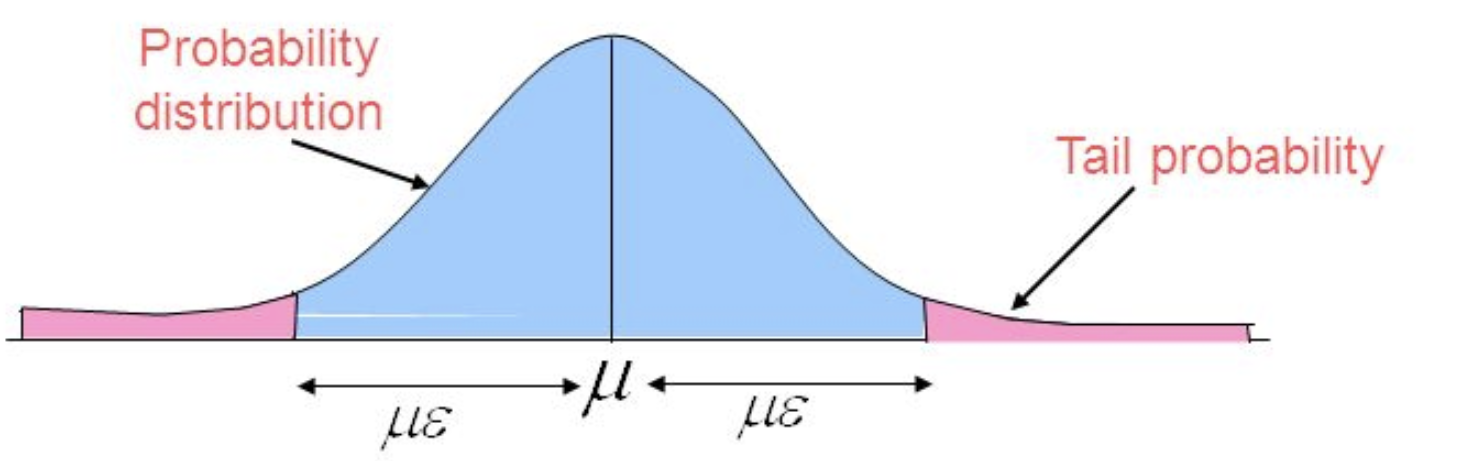
  • Key Idea: very often most of the probability is concentrated among small proportion of sample space
  • Bound probability that random variable with bell-shaped distribution takes value in tails of the distribution, i.e., far away from the mean.

Markov's Inequality

"No more than 1/5 of the population can have more than 5 times the average income."
  • The most basic concentration bound
  • Requires (almost) no knowledge about properties of random variable
  • Consequently, the bound isn't very tight
  • Nevertheless many applications
Theorem: If X is a nonnegative (discrete) RV and a > 0 , then: \Pr{ X \ge a \cdot \EE{X}} \le \frac{1}{a}

Proof by Picture! :-)

  • \color{blue}{g(x)} = x
  • \color{green}{f(x)} = \begin{cases} 0 &\text{$x < a\Ee{X}$} \\ a\Ee{X} &\text{$x\ge a\Ee{X}$} \end{cases}
  • \Ra \forall x\colon f(x) \le g(x)
  • Define p(x) = \Pr{ X = x}
\Ra\ \fragment{a\Ee{X}\cdot \Pr{X\!\ge\! a \Ee{X}} =} \sum_{x} f(x)p(x) \le \sum_x g(x)p(x) \fragment{= \Ee{X}}

Proof by Algebra:

  • \begin{align} (a\Ee{X}) \cdot \Pr{X \ge a\cdot \EE{X}\ } &= (a\Ee{X})\cdot \sum_{k\ge a \Ee{X}} \Pr{X=k}\\ &\fragment{ = \sum_{k\ge a\Ee{X}} (a\Ee{X})\cdot \Pr{X=k} }\\ &\fragment{ \le \sum_{k\ge a\Ee{X}} \color{red}{k} \cdot \Pr{X=k} }\\ &\fragment{ \le \sum_{k\in\range(X)} k \cdot \Pr{X=k} } \fragment{ = \Ee{X} } \end{align}
  • \Ra \Pr{ X \ge a \cdot \EE{X}} \le \tfrac{\Ee{X}}{a\Ee{X}}

Revisiting Distributed MIS Algorithm

  • So far, we obtained O(\log n) expected number of rounds.
  • Recall:
Lemma: After iteration m=\lceil 4\log_2 n\rceil , it holds: \expect{ L_m } \le \tfrac{10}{n^2}

Idea: Apply Markov's Inequality to RV L_m , since L_m > 0 .

Lemma: If X is a nonnegative (discrete) RV and a > 0 , then: \Pr{ X \ge a \cdot \EE{X}} \le \frac{1}{a}
  • \Pr{ L_m \ge 1 } \le \EE{ L_ m } \le \tfrac{10}{n^2}
  • Algorithm terminates within \lceil 4n\log_2 n\rceil iterations with probability \ge 1 - O\left(\tfrac{1}{n^2}\right) : For n=20 , this is \ge 0.9975

Revisiting Byzantine Agreement

Lemma: The Randomized Byzantine Agreement Algorithm terminates in 3 rounds in expectation.
  • Let T be RV of number of rounds of algorithm.
  • \Ra \Pr{ T\ge x } \le \frac{\Ee{T}}{x}
  • To get probability p , solve right-hand side for x :
  • \tfrac{\Ee{T}}{x} \le 1-p

Example:

  • For p=0.9 : x = \Ee{T}/0.1 = 30
  • For p=0.99 : x = \Ee{T}/0.1 = 300

Expectation alone might not be Sufficient

Consider the following coin flipping games

  1. You flip one fair coin. You win $1 if heads; you lose $1 if tails.
  2. You flip 10 fair coins. You win $1000 if all heads; else you lose $1

Let's compute expected value of winnings X :

  • Game 1: \EE{X} = \tfrac{1}{2}\cdot 1 + \tfrac{1}{2}\cdot (-1) = 0
  • Game 1: \EE{X} = \tfrac{1}{2^{10}}\cdot 1000 + (1-\tfrac{1}{2^{10}})\cdot (-1) \approx 2
  • Which game would you prefer?

Variance

Definition: Consider RV X . The variance \var{X} is the expectation of squared deviation of RV X from \Ee{X} : \var{X} = \EE{(X - \EE{X})^2}
  • Red distribution has mean 100 and variance 100 ( SD=10 )
  • Blue distribution has mean 100 and variance 2500 ( SD=50 )
(source: wikipedia)
image/svg+xml

Example: Variance of Fair Coin Flip

  • Let X be indicator random variable of fair coin flip. Then:
  • \Pr{X=0} = \Prob{X=1} = \tfrac{1}{2} .
  • \Ee{X} = \tfrac{1}{2} .
  • What about Variance? \begin{align} \var{X} &= \EE{(X - \EE{X})^2} \\ &\fragment{ = \sum_{k\in\range{(X-\Ee{X})}} k\cdot \Prob{(X-\Ee{X})=k} }\\ &\fragment{ = \sum_{k\in\range{(X-\color{red}{\tfrac{1}{2}})}} k\cdot \Prob{(X-\color{red}{\tfrac{1}{2}})=k} }\\ &\fragment{ = \brackets{1 - \tfrac{1}{2}}^2\cdot\tfrac{1}{2} \fragment{+ \brackets{0 - \tfrac{1}{2}}^2\cdot\tfrac{1}{2}} } \fragment{ = \tfrac{1}{4} } \end{align}

Expectation of Product of Independent RVs

Lemma: If X and Y are independent RVs, then: \EE{X \cdot Y} = \EE{X} \cdot \EE{Y}.

Proof:

  • \begin{align} \EE{X Y } &= \sum_{i} \sum_j i \cdot j \cdot \Pr{X = i, Y = j} \\ &\fragment{ = \sum_{i} \sum_j i \cdot j \cdot \Pr{X = i} \cdot \Pr{Y = j} \\ }\\ &\fragment{ = \sum_{i} i \cdot \Pr{X = i} \cdot \sum_j j \cdot \Pr{Y = j} \\ }\\ &\fragment{ = \EE{X} \cdot \EE{Y} } \end{align}

Linearity of Variance of Independent RVs

Lemma: If X and Y are independent RVs, then: \Var{X + Y} = \Var{X} + \Var{Y}

Proof:

  • \begin{align} \Var{X + Y } &= \EE{(X + Y - \EE{X+Y})^2}\\ &\fragment{ = \EE{((X - \EE{X}) + (Y - \EE{Y}))^2} }\\ &\fragment{ = \EE{(X - \EE{X})^2 + (Y - \EE{Y})^2 + 2(X - \EE{X})(Y-\EE{Y})} }\\ \end{align}
  • But \EE{X - \EE{X}} = \fragment{\EE{X} - \EE{\EE{X}} = \EE{X} - \fragment{\EE{X} = 0.}}
  • Therefore: \Var{X + Y } = \EE{(X - \EE{X})^2 + (Y - \EE{Y})^2} = \Var{X} + \Var{Y}

Plan for Today

  • Bernoulli & Binomial RVs
  • Algorithm for Computing Median
  • Chernoff Bounds (maybe Tuesday)

Chebyshev's Inequality

Theorem: For any random variable X and any a>0 : \Pr{|X - \Ee{X}|\! \ge\! a} \le \frac{\var{X}}{a^2}

Proof:

  • Just use Markov's Inequality:
  • Define helper RV Y = (X - \Ee{X})^2
  • \begin{align} \Pr{|X - \Ee{X}|\! \ge\! a} &\fragment{\, = \Pr{(X - \Ee{X})^2\! \ge\! a^2} }\\ &\fragment{\, = \Pr{Y \ge a^2} \le \tfrac{\expect{Y}}{a^2} } \fragment{ = \frac{\Var{X}}{a^2} } \end{align}

Bernoulli Random Variables

Indicator RV X is a Bernoulli RV with parameter p , denoted X \sim \text{Brn}(p) , if \Pr{X=1} = p and \Pr{X=0}=1-p .
  • Example: Fair coin flip is Bernoulli RV with parameter \tfrac{1}{2} . Indicator RVs!

General Properties:

  • Expectation: \EE{X} = \Pr{X=1} = {p}
  • Variance calculated similarly as for fair coin flip: \begin{align} \Var{X} &= \EE{(X-p)^2} \\ &= (0-p)^2\cdot p + (1-p) \cdot (1-p) = p(1-p). \end{align}

Binomial Random Variables

Let X_1,\dots,X_n be n independent Bernoulli RVs with parameters p and define X = \sum_{i=1}^n X_i . Then X is a Binomial RV with parameters n and p , denoted X \sim \text{Binom}(n,p) , such that: \Pr{X \!=\! k} = {n \choose k} p^k (1 - p)^{n-k}

General Properties:

  • Computing expectation and variance is straightforward!
  • \EE{X} = \EE{\sum_{i=1}^n X_i} = \sum_{i=1}^n\EE{X_i} = \sum_{i=1}^n p = n p
  • \Var{X} = \Var{\sum_{i=1}^n X_i} = \sum_{i=1}^n \Var{X_i} = \sum_{i=1}^n p(1-p) = n p(1-p)

Fast Computation of the Median

  • We're given some unsorted data set: list of n integers
  • Median is the value separating the higher half from the lower half of the data set
  • m is median, if...
    1. at least \lfloor n/2 \rfloor elements are \le m , and
    2. at least \lfloor n/2 \rfloor + 1 elements are \ge m .
  • Goal: Output the median element in time O(n) (in RAM model)
  • 4
    4
    1
    1
    3
    3
    9
    9
    8
    8
    4
    4
    2
    2
    7
    7
    8
    8
    0
    0
    6
    6
    9
    9
    6
    6
    median:
    4
    4
    1
    1
    3
    3
    9
    9
    8
    8
    4
    4
    2
    2
    7
    7
    8
    8
    0
    0
    6
    6
    6
    6
    9
    9
  • Easy way to compute median in time O(n\log n) ?
  • Sort list and output middle element in sorted order

Why the median is important

  • Consider sample of 1000 household incomes
  • Let's assume all except 1 sample earn 80,000\$ .
  • One sample earns 158.2 billion USD (e.g. CEO of Amazon.com)
  • Value of Mean? \approx 158,000,000\$
  • Value of Median? 80,000\$
  • Median is more robust to outliers!

Randomized Algorithm for Median - High Level

  • Input: List S of n = 2k+1 integers; n odd
  • Output: median of S , i.e.: (k+1) -th element in sorted order of S
  • Main Idea:

    • Sampling of small subsets
    • ...and sorting of small subsets

Randomized Algorithm for Computing Median

Input: Unsorted array S of n integers;

Output: median m of S

  1. Sample \lceil n^{3/4} \rceil elements u.a.r from S . Store them in array R .
  2. R' \gets \text{Merge-Sort}(R)
  3. a \gets R'\!\left[\lfloor \tfrac{1}{2}n^{3/4} - \sqrt{n}\rfloor\right]
  4. b \gets R'\!\left[\lfloor \tfrac{1}{2}n^{3/4} + \sqrt{n}\rfloor\right]
  5. C \gets \set{ x \in S\colon a \le x \le b }
  6. \alpha \gets |\set{x \in S\colon x < a}
  7. \beta \gets |\set{x \in S\colon x > b}
  8. if (\alpha > n/2) or (\beta > n/2) then: output fail and terminate
  9. if |C| > 4n^{3/4} then: output fail and terminate
  10. C' \gets \text{Merge-Sort}(C)
  11. output C'\!\left[\lfloor n/2 \rfloor - \alpha + 1\right]
Intuition

Find a and b such that:

  1. a \le m \le b
  2. |C| = O(n/\log n)
Lemma: The algorithm terminates in time O(n) and outputs either fail or the median.

Proof:

Time Complexity:

  • Sorting R takes O(|R|\log |R|) = O(n^{3/4}\log(n^{3/4})) = o(n) .
  • Computing C , \alpha , \beta , takes O(n) , i.e., each time 1 pass through S .
  • Sorting C takes O(|C|\log |C|) = O(n^{3/4}\log(n^{3/4})) = o(n) .
  • \Ra O(n) time in total.

Correctness:

  • Algorithm is correct if it either outputs fail or median.
  • Suppose algorithm outputs m' . Is m' median?
  • We know a \le m' \le b ; otherwise algorithm would have output fail
  • \Ra m' \in C
  • \Ra m' = C'\!\left[ \lfloor n/2\rfloor - \alpha + 1\right] (this is only element that is output)
  • Exactly \alpha elements less or equal than a
  • \Ra C' doesn't contain smallest \alpha elements of S
  • \Ra element m' at position \lfloor n/2\rfloor - \alpha + 1 of C' is median of S .

Analysis of Success Probability
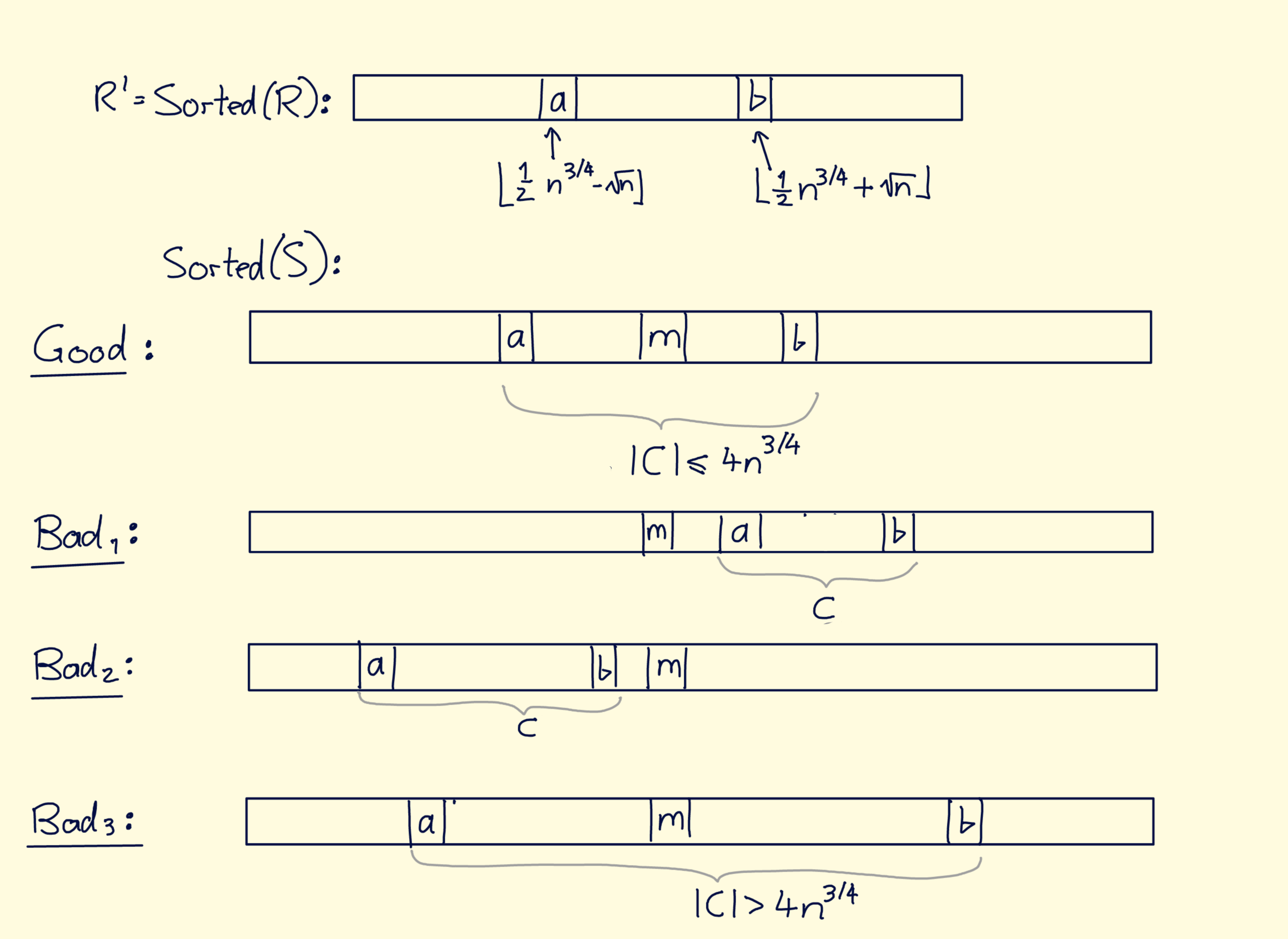
We need to avoid 3 bad events...
  • \bad_1 : occurs if \alpha > \tfrac{n}{2}
  • \bad_2 : occurs if \beta > \tfrac{n}{2}
  • \bad_3 : occurs if |C| > 4n^{3/4}
Lemma: \Pr{\bad_1} = \Pr{ \alpha\!>\! \tfrac{n}{2} } < \frac{1}{4n^{1/4}} .

Proof:

  • \bad_1 occurs...
    • \Leftrightarrow a > m
    • \Leftrightarrow |\set{r \in R\colon r\le m}| < \tfrac{1}{2}n^{3/4} - \sqrt{n}
    • \phantom{\Leftrightarrow} because m cannot be greater than (\tfrac{1}{2}n^{3/4}\!-\!\sqrt{n} ) smallest elements of R
  • Define X_i = \begin{cases} 1 & \text{if $i$-th sample of $R$ is $\le m$}\\ 0 & \text{otherwise} \end{cases}
  • \Ra \E{X_i} = \Pr{X_i = 1} = \tfrac{\text{# elem. in $S$ that $\le m$}}{n} = \tfrac{(n-1)/2+1}{n} = \frac{1}{2}+\frac{1}{2n}
  • Define Y = \sum_{i=1}^{|R|} X_i
  • \Ra \Pr{\bad_1} = \Pr{ Y < \tfrac{1}{2} n^{3/4} - \sqrt{n}}
  • \Pr{\bad_1} = \Pr{ Y < \tfrac{1}{2} n^{3/4} - \sqrt{n}}
  • Idea: Use Chebyshev's Inequality!
  • First determine \E{Y} and \Var{Y} ...
  • Since Y \sim \text{Binom}(|R|,\tfrac{1}{2} + \tfrac{1}{2n}) :
    • \E{Y} = \sum_{i=1}^{|R|} \E{X_i} = n^{3/4}\lb( \tfrac{1}{2} + \tfrac{1}{2n}\rb) = \tfrac{1}{2}n^{3/4} + \tfrac{1}{2n^{1/4}} > \tfrac{1}{2}n^{3/4}
    • \Var{Y} = n^{3/4}\lb( \tfrac{1}{2} + \tfrac{1}{2n}\rb) \lb(1 - \tfrac{1}{2} - \tfrac{1}{2n}\rb) = \tfrac{1}{4}n^{3/4} - \tfrac{1}{4n^{5/4}} < \tfrac{1}{4}n^{3/4}
  • \E{Y} > \tfrac{1}{2}n^{3/4}
  • \Var{Y} < \tfrac{1}{4}n^{3/4}
  • Now let's apply Chebyshev's Inequality:
\begin{align} \Pr{ Y < \tfrac{1}{2} n^{3/4} - \sqrt{n}} &= \Pr{ Y - \tfrac{1}{2} n^{3/4} < - \sqrt{n}} \\ &\fragment{\, = \Pr{ \tfrac{1}{2} n^{3/4} - Y > \sqrt{n}} }\\ &\fragment{\, \le \Pr{ |\tfrac{1}{2} n^{3/4} - Y| > \sqrt{n}} }\\ &\fragment{\, \le \frac{\var{Y}}{(\sqrt{n})^2} } \fragment{\, < \frac{\tfrac{1}{4}n^{3/4}}{n} } \fragment{\, = \frac{1}{4n^{1/4}} } \end{align}
Lemma: \Pr{\bad_2} = \Pr{ \beta\!>\! \tfrac{n}{2} } < \frac{1}{4n^{1/4}} .

Proof:

  • Same analysis as for \Pr{\bad_1} .
Lemma: \Pr{ \bad_3 } = \Pr{ |C| > 4n^{3/4}} < \frac{1}{2n^{1/4}}

Proof:

  • Define 2 events:
    1. Event A : at least |C|/2 = 2n^{3/4} elements of C are \ge m
    2. Event B : at least |C|/2 = 2n^{3/4} elements of C are \le m
  • If |C| > 4n^{3/4} , then at least one of A or B occurs.
  • Focus on event A : at least |C|/2 = 2n^{3/4} elements of C are \ge m . (Argument for B is symmetric.)
  • Recall that b \ge x for all x \in C .
  • \Ra event A implies that position of b in \text{Sorted}(S) is \ge \tfrac{1}{2}n + 2n^{3/4}
  • Define X_i = \begin{cases} 1 & \text{$i$-th sample is among $\tfrac{1}{2}n-2n^{3/4}$ largest of $S$}\\ 0 & \text{otherwise} \end{cases}
  • \EE{X_i} = \Pr{X_i=1} = \tfrac{(1/2)n - 2n^{3/4}}{n} = \tfrac{1}{2} - \tfrac{2}{n^{1/4}}
  • Define X = \sum_i^{|R|} X_i . Then X \sim \text{Binom}(n^{3/4},\tfrac{(1/2)n - 2n^{3/4}}{n})
  • Define X = \sum_i^{|R|} X_i . Then X \sim \text{Binom}(n^{3/4},\tfrac{1}{2} - \tfrac{2}{n^{1/4}}) and thus:
    • \EE{X} = n^{3/4}\brackets{\tfrac{1}{2} - \tfrac{2}{n^{1/4}}} = \tfrac{1}{2}n^{3/4} - 2\sqrt{n}
    • \Var{X} = n^{3/4} \brackets{\tfrac{1}{2} - \tfrac{2}{n^{1/4}}} \brackets{1 - \brackets{\tfrac{1}{2} - \tfrac{2}{n^{1/4}}}} = \frac{1}{4}n^{3/4} - 4n^{1/4} < \tfrac{1}{4} n^{3/4}
  • Let's apply Chebyshev's Inequality:
  • \begin{align} \Pr{A} = \Pr{ X \ge \tfrac{1}{2}n^{3/4} - \sqrt{n}} &\fragment{ = \Pr{ X \ge \tfrac{1}{2}n^{3/4} - \color{red}{2}\sqrt{n} + \color{red}{\sqrt{n}}} }\\ &\fragment{ = \Pr{ X - \EE{X} \ge \sqrt{n}} }\\ &\fragment{ \le \Pr{ |X - \E{X}| \ge \sqrt{n}} }\\ &\fragment{ \le \frac{\var{X}}{n} \fragment{=\tfrac{1}{4n^{1/4}}} } \end{align}
  • Recall that event \bad_3 happens if event A or B
  • So far, we've shown that \Pr{A} \le \tfrac{1}{4n^{1/4}} .
  • Symmetric argument shows that \Pr{B} \le \tfrac{1}{4n^{1/4}} .
  • \Ra \Pr{\bad_3} \le \Pr{A} + \Pr{B} \le \tfrac{1}{2n^{1/4}} .

Combining All the Pieces

  • Algorithm outputs median unless \bad_1 or \bad_2 or \bad_3 happen.
  • \begin{align} \Ra \Pr{\texttt{fail}} &\le \Pr{\bad_1} + \Pr{\bad_2} + \Pr{\bad_3} \\ &\fragment{ \le 2 \cdot \tfrac{1}{4n^{1/4}} + \tfrac{1}{2n^{1/4}} }\\ &\fragment{ = \tfrac{1}{n^{1/4}} } \end{align}
Theorem: There exists a randomized Monte Carlo algorithm that runs in time O(n) and outputs the median for a given input array of n integers with probability at least 1 - \tfrac{1}{n^{1/4}} .

Can we make this a Las Vegas algorithm?

Interlude: Probability vs Logical Implications

  • Consider events A and B .
  • " A \Ra B " implies \Pr{A} \le \Pr{B} .
  • Why?
    • Recall: an event is set of outcomes
    • So A \Ra B really means, for all outcomes x \in A , also x \in B
    • Thus A \subseteq B
    • Probability of set B cannot be smaller than probability of set A .
  • Example: {x-y > d} \Ra {|x-y|>d} , so \Pr{ x-y > d} \le \Pr{ |x-y| > d}

Chernoff Bounds

  • Tail inequality for random variables
  • Gives much tighter bounds than Markov's or Chebyshev's Ineq.
  • Extremely common tool when analyzing stochastic processes and algorithms

General Version of Chernoff Bound

Theorem (General Version): Let X_1,\dots,X_n be independent Bernoulli RVs with parameter p and define X = \sum_{i=1}^{n}X_i .
For any \delta >0 : \Pr{X \ge (1+\delta) \EE{X} } \le \br{ \frac{e^\delta}{(1+\delta)^{1+\delta}}}^{\E{X}} For any \delta \in (0,1) : \Pr{X \le (1-\delta) \EE{X} } \le \br{ \frac{e^{-\delta}}{(1-\delta)^{1-\delta}}}^{\E{X}}

Simplified Version of Chernoff Bound

Theorem (Simplified Version): Let X_1,\dots,X_n be independent Bernoulli RVs with parameter p and define X = \sum_{i=1}^{n}X_i .
For any \delta \in (0,1) : \Pr{X \ge (1+\delta)\EE{X}} \le e^{-\Ee{X}\cdot \delta^2 / 3} \Pr{X \le (1-\delta) \EE{X} } \le e^{-\Ee{X}\cdot \delta^2 / 3}

Example: Concentration Bounds for Coin Flips

  • n fair coins, i.e., \Prob{X_i = 1} = \tfrac{1}{2} . Define X = \sum_{i=1}^n X_i .
  • We already know \EE{X} = \tfrac{n}{2} , \Var{X} = \tfrac{n}{4} .

What's the probability of seeing more than \tfrac{3}{4}n heads?

Let's use Markov's Inequality: \Pr{X \ge a\EE{X}} \le \tfrac{1}{a} :
  • \Pr{ X \ge \tfrac{3}{4}n} = \Pr{ X \ge \tfrac{6}{4}\tfrac{n}{2}} \le \frac{1}{(6/4)} = \frac{2}{3}
  • Not very useful here...
Let's use Chebyshev's Inequality: \Pr{|X - \EE{X}| \ge a} \le \tfrac{\var{X}}{a^2}
  • \begin{align} \Pr{ X \ge \tfrac{3}{4}n} &= \Pr{ X - \color{red}{\EE{X}}\ge \tfrac{3}{4}n -\color{red}{\EE{X}}} \\ &\fragment{ = \Pr{ X - \EE{X} \ge \tfrac{1}{4}n} }\\ &\fragment{ \le \Pr{ |X - \EE{X}| \ge \tfrac{1}{4}n} } \fragment{ \le \frac{\var{X}}{(n/4)^2} \fragment{ = \frac{n/4}{(n/4)^2} } \fragment{ = \frac{4}{n} } } \end{align}
  • We got a tighter bound, but we can still do better!
Let's use Chernoff Bound: \Pr{X\ge (1+\delta)\EE{X}} \le \exp\br{\tfrac{-\delta^2 \Ee{X}}{3}}
  • \begin{align} \Pr{X \ge \tfrac{3}{4}n} &\fragment{ = \Pr{ X \ge (1 + \tfrac{1}{2})\tfrac{n}{2}} }\\ &\fragment{ \le e^{-\br{\tfrac{1}{2}}^2\tfrac{n}{2}\tfrac{1}{3}} } \fragment{ \le e^{-n/24} } \end{align}
  • \Ra Decreases exponentially in n ! Very unlikely event.

Can we get even closer to the mean?

Again: Use Chernoff Bound \Pr{X\ge (1+\delta)\EE{X}} \le \exp\br{\tfrac{-\delta^2 \Ee{X}}{3}}
  • \Pr{X \ge \EE{X} \color{red}{+ \lambda} } = \Pr{ X \ge \br{1 + \tfrac{\lambda}{\Ee{X}}} \EE{X}} , so \delta = \tfrac{\lambda}{\Ee{X}} .
  • Choose \lambda = \sqrt{6 \EE{X}\log n }
\Pr{ X \ge \tfrac{n}{2} + \sqrt{6 n \log n} } \le \exp\br{ -\br{\tfrac{\lambda}{\Ee{X}}}^2\Ee{X}/3} = \exp\br{-\tfrac{6\Ee{X}\log n}{(\Ee{X})^2} \Ee{X}/3} = \tfrac{1}{n^2}
  • Observing \tfrac{n}{2}+\epsilon n heads is unlikely for any constant \epsilon >0 !

Revisiting Randomized Quicksort

qsort(array): 
 if length(array) ≤ 1 then
   return array
 else
   pivot = array[random(0..length(array))] 
   less_or_eq = [ x <- array | x ≤ pivot ]
   greater = [ x <- array | x > pivot ]
   qsort(less_or_eq) ++ [pivot] ++ qsort(greater)
Theorem: Randomized Quicksort runs in O(n\log n) time with high probability.

Proof:

  • View execution of quicksort as binary tree:
    • Root of tree is initial data set S
    • Left child is subproblem of sorting elements smaller than pivot
    • Right child is subproblem of sorting elements greater than pivot
    • Each internal node of tree is subproblem of smaller size
    • Each leaf corresponds to singleton set
  • Node x of tree is good if subproblem of both children is at most \tfrac{2}{3} of x 's problem size.
  • 2 Simple Properties:
    1. \Pr{\text{node is good}} = \frac{1}{3}
    2. Number of good nodes in any path from root to leaf is at most \log_{3/2} n .
1. \Pr{\text{node is good}} = \frac{1}{3}
  • Consider sorted order S' of m \le n integers at some node x .
\begin{align} \Pr{\text{node $x$ is good}} &\fragment{= 1- \Pr{ \text{pivot neither in smallest nor largest $\tfrac{1}{3}$}}} \\ &\fragment{= 1 - (\Pr{ \text{pivot not in smallest $\tfrac{1}{3}$}} + \Pr{ \text{pivot not in largest $\tfrac{1}{3}$}} )} \\ &\fragment{= 1 - 2\frac{1}{3} = \frac{1}{3}} \end{align}
2. Number of good nodes in any path from root to leaf is at most \log_{3/2} n .
  • Good node reduces problem size by \left(\tfrac{2}{3}\right) -fraction.
  • If path contains k good nodes, then...
  • problem size \le \lb(\frac{2}{3}\rb)^k n
  • \Ra problem size of 1 for k = \log_{3/2}(n) .
  • Consider a path \Gamma of length |\Gamma| = 48\log_{3/2}n .
  • Define indicator RV X_i = 1 iff i -th node in p is good
  • Define X = \sum_{i=1}^{|\Gamma|}X_i . Then \E{X} = |\Gamma| \tfrac{1}{3} = 16 \log_{3/2} n .
\begin{align} \Pr{ X \le \log_{3/2}n} &\fragment{\, \le \Pr{ X \le \lb(1-\tfrac{1}{2}\rb)\cdot 16\log_{3/2}n} \qquad\text{($\delta=\tfrac{1}{2}$)} } \\ &\fragment{\, \le \exp\lb( -\frac{\lb(\tfrac{1}{2}\rb)^2 16\log_{3/2}n}{3} \rb) }\\ &\fragment{\, = \exp\lb(-\tfrac{4}{3}\log_{3/2} n\rb) } \fragment{\, \le \exp(-2\log n) } \fragment{\, = \frac{1}{n^2} } \end{align}
  • We've shown: \Pr{ \text{$\exists$ path of length $\ge 48\log n$ containing $\le \log_{3/2}(n)$ good nodes}} \le \frac{1}{n^2}
  • We've shown: p := \Pr{ \text{$\exists$ path of length $\ge 48\log n$ containing $\le \log_{3/2}(n)$ good nodes}} \le \frac{1}{n^2}
  • Take union bound over all n paths: \Pr{ \text{any of $n$ paths of length $\ge 48\log n$ has $\le \log_{3/2}(n)$ good nodes}} \le \fragment{n p = \frac{1}{n}}
  • \Ra No path has length \ge 48\log n .
Theorem: Randomized Quicksort runs in O(n\log n) time with high probability.

Application: Sampling & Polling

"What fraction of CAS alumni like Haskell?"
  • Suppose we have s samples from the population of CAS alumni.
  • p -fraction of CAS alumni like Haskell, where p is unknown
  • Its impossible to find p exactly, so let's try to find "likely range":
  • Goal: To have "confidence" 1-\gamma , we need interval I such that \Pr{ p \in I } \ge 1 - \gamma
Def: A (1 - \gamma) confidence interval of size \delta for parameter p is an interval [q - \delta, q + \delta] such that: \Pr{ p \in [q - \delta,q+\delta]\ } \ge 1 - \gamma
  • We want s to be as small as possible!
Def: A (1 - \gamma) confidence interval for parameter p is an interval [q - \delta, q + \delta] such that: \Pr{ p \in [q - \delta,q+\delta]\ } \ge 1 - \gamma
  • Let X be # of sampled alumni that like Haskell.
  • Then X = s q , for some q \in [0,1] . Important: likely that q \ne p !
  • Also: X \sim \text{Binom}(s,\color{red}{p}) and \E{X} = s {p} .
  • If p \notin [q - \delta,q+\delta] then either:
    1. p < q - \delta , hence \color{blue}{X} = s q \color{blue}{>} s (p+\delta) \fragment{= s p(1+\delta/p) } \fragment{= \color{blue}{\E{X}(1+\delta/p)} }
    2. p > q + \delta , hence \color{blue}{X} = s q \color{blue}{<} s (p-\delta) \fragment{= s p(1-\delta/p) } \fragment{= \color{blue}{\E{X}(1-\delta/p)} }
\begin{align} \Pr{ p \notin [q - \delta, q + \delta]} = \Pr{ X < sp(1+\delta/p)} + \Pr{ X > sp(1-\delta/p)} \end{align}
\begin{align} \Pr{ p \notin [q - \delta, q + \delta]} &= \Pr{ X < sp(1+\delta/p)} + \Pr{ X > sp(1-\delta/p)} \\ &\fragment{\, \le e^{-sp(\delta/p)^2/3} + e^{-sp(\delta/p)^2/3} }\\ &\fragment{\, = 2e^{-s\delta^2/(2p)} }\\ &\fragment{\, \le 2e^{-s\delta^2/2} \qquad \text{(since $p\le 1$)} } \end{align}
  • We want \Pr{ p \notin [q - \delta, q + \delta]} < \gamma , so we set: \begin{align} \gamma &= 2e^{-s\delta^2/2} \end{align}
  • If we fix \gamma and \delta , how many samples do we need to get (1-\gamma) -confidence interval of size \pm \delta ?
  • \begin{align} &\fragment{\, \Ra s = \frac{\log\lb( \tfrac{4}{\gamma^2}\rb)}{\delta^2} } \end{align}
    If \delta and \gamma are constant: s is independent of population size! Works just as well when sampling from population of China.

Final Projects

  • When designing new randomized algorithm, there's interplay between theory and experiment.
  • From theory, we get insights what might work in practice
  • From experiments, we can see what we should try to prove
  • Goal of final project: To perform experiments with randomized algorithms.

Project Topics

  • 3 topics: choose one to work on
  • You can also suggest a different topic if it is related to the course.
  • Write a report on your findings.
  • Give a brief presentation in class.

Topic 1: Quicksort with Multiple Pivots

  • Standard randomized quicksort uses 1 pivot element at each recursive step to split elements into 2 smaller sets.
  • In 2009, researchers obtained faster results using two pivots that split elements into 3 smaller sets.
  • Implement (standard) randomized Quicksort and multi-pivot Quicksort.
  • Perform baseline performance measurements (count number of comparisons!).
  • How many pivots is optimal?
  • What about parallelizing your implementation?
  • How does the running time of your implementation scale with n ?
  • Try to use different data sets: almost pre-sorted,

Topic 2: Skip Lists vs Binary Search Trees

  • Skip lists are an interesting alternative to binary search trees.
  • Goal is to understand performance of skip lists compared to other (randomized or deterministic) data structures.
  • Implement skip lists, treaps, and red-black trees.
  • Perform baseline performance measurements.
  • Which data structures perform best for which sequence of operations? Why?
  • Use variety of data sets!

Topic 3: Contention Resolution

  • One of the most frequent uses of randomization in real world
  • Scenario: collection of devices/processes want to access some resource
  • Resource can only be accessed by one user at a time (e.g. collision resolution in 802.11 WiFi)
  • Assume that time proceeds in synchronous steps 1,2,... .
  • In each step, a device can attempt to claim the resource.
  • If it succeeds, then it completes. Otherwise, it backs off and tries again later.
  • Backoff protocol determines time-window for retry.
  • Goal: Experiment with Backoff Protocols
  • Many variants: Linear backoff, exponential backoff, log-backoff, etc.
  • Implement simple simulator that can run different backoff protocols
  • Which backoff protocol works best? Under what circumstances?

Skip Lists

Geometric Random Variables

Consider experiment that succeeds with probability p and fails with probability 1-p . Let RV X be number of trials until first success. Then X is a geometric RV with parameter p and: \forall i\ge 1\colon\ \Pr{ X \!=\! i } = (1 - p)^{i-1}\cdot p

Properties

  • \sum_{i\ge 1} \Pr{X \!=\! i} = \sum_{i\ge 1} (1 - p)^{i-1}p = p\cdot \frac{1}{1 - (1-p)} = 1
  • Memoryless: Past failures do not change distribution of number of trials until first success.

The Memoryless Property

Lemma: Consider geometric RV X . Then, for any positive integers k , n : \Pr{ X = n+k \mid X>k } = \Pr{ X = n}

Proof:

  • \begin{align} \Pr{ X = n+k \mid X >k } &=\frac{\Pr{ (X = n+k) \cap (X >k) }}{\Pr{X>k}} \\ &\fragment{\, = \frac{\Pr{ X = n+k }}{\Pr{X>k}} }\\ &\fragment{\, = \frac{(1-p)^{n+k-1}p}{\Pr{X>k}} }\\ &\fragment{\, = \frac{(1-p)^{n+k-1}p}{\sum_{i\ge k+1}(1-p)^{i-1}p} } \end{align}
  • \begin{align} \Pr{ X = n+k \mid X >k } &= \frac{(1-p)^{n+k-1}p}{\sum_{i\ge k+1}(1-p)^{i-1}p} \\ &\fragment{ = \frac{(1-p)^{n+k-1}p}{p\sum_{i\ge k}(1-p)^{i}} }\\ &\fragment{\, = \frac{(1-p)^{n+k-1}p}{p (1-p)^k\sum_{i\ge 0}(1-p)^{i}} }\\ &\fragment{\, = \frac{(1-p)^{n+k-1}p}{p (1-p)^k\tfrac{1}{1-(1-p)}} } \fragment{\, = (1 - p)^{n-1}p } \fragment{\, = \Pr{ X = n} } \end{align}

Expectation of Nonnegative Random Variable

Theorem: Let X be a discrete random variable that takes on only nonnegative values. Then \E{X} = \sum_{i= 1}^{\infty}\Pr{ X\ge i} .

Proof:

  • \begin{align} \sum_{i= 1}^{\infty}\Pr{ X\ge i} &\fragment{\, = \sum_{i= 1}^{\infty} \lb(\sum_{j=i}^{\infty} \Pr{ X =j } \rb) }\\ &\fragment{\, = \sum_{j=1}^{\infty} \sum_{i= 1}^{j} \Pr{ X =j } }\\ &\fragment{\, = \sum_{j=1}^{\infty} j\cdot \Pr{ X =j } } \fragment{\, = \E{X} } \end{align}

Expectation of Geometric Random Variable

Theorem: Let X be a geometric RV with parameter p . Then \E{X} = \frac{1}{p} .

Proof:

  • Let's use \E{X} = \sum_{i= 1}^{\infty}\Pr{ X\ge i} .
  • \begin{align} \Pr{ X \ge i } = \sum_{n=i}^{\infty} (1 - p)^{n-1} p &\fragment{\, = p \cdot \sum_{n=\color{red}{i-1}}^{\infty} (1 - p)^{n} }\\ &\fragment{\, = p \cdot (1 - p)^{i-1} \sum_{n=\color{red}{0}}^{\infty} (1 - p)^{n} }\\ &\fragment{\, = p \cdot (1 - p)^{i-1} \tfrac{1}{1-(1-p)} } \fragment{\, = (1 - p)^{i-1} }\\ \end{align}
  • So far: \Pr{ X \ge i } = (1 - p)^{i-1} .
  • \begin{align} \E{X} &= \sum_{i=1}^{\infty} \Pr{X \ge i} \\ &\fragment{\, = \sum_{i=1}^{\infty} (1 - p)^{i-1} }\\ &\fragment{\, = \sum_{i=0}^{\infty} (1 - p)^{i} } \fragment{\, = \frac{1}{1-(1-p)} } \fragment{\, = \frac{1}{p} } \end{align}

The Data Structuring Problem

  • Given collection C of n data items: (k_1,\text{item}_1),\dots,(k_n,\text{item}_n)
  • Each item has unique key k_i
  • Goal: Maintain keys of C in a way that supports insert, search, delete in time O(\log n) .
  • Standard Solution: represent keys in binary search tree.

Example

Keys \{1,3,4,6,7,8,10,14,13\}

Deterministic Binary Search Trees

  • Deterministic solution to data structuring problem
  • O(\log n) time operations if tree is balanced:

    Performance is proportional to height of tree!

  • Worst-case insertion sequences requires rebalancing of tree.

Example: Red-Black Tree

  • Most popular self-balancing binary tree
  • Each node has color: either red or black.
  • Red nodes have only black children
  • All paths from a node to leaf have same number of black nodes

Rebalancing Red-Black Tree

  • Maintaining invariants requires rotations
  • Might affect large parts of the tree: problematic when data is partitioned across several machines
  • Implementing concurrent write-access to elements is tricky

Deterministic Variant of Skip Lists

One-Shot Construction
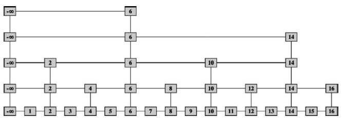
  • Consider ordered collection of keys C = \{k_1,k_2,\dots,k_n\} .
  • Build level 0 linked list L_0 = (-\infty \ra k_1 \ra k_2 \ra \cdots \ra k_n) .
  • Build level 1 linked list L_1 = (-\infty \ra k_2 \ra k_4 \ra \cdots \ra k_{m})
  • Add double pointers between identical elements in L_0 and L_1 .
  • Build level i linked list L_i by omitting every second key from L_{i-1} ; add double pointers between identical elements
  • Elements in L_0 hold reference to stored items of respective keys.
  • L_t is called top list
  • We get \lceil \log_2 n\rceil distinct linked lists L_0,\dots,L_t .

Example: Skip List of keys \{1,\dots,16\}

Searching in Skip Lists

Suppose we search for key y :

  1. Start at left-most element in top list L_t .
  2. Scan right until we hit largest element e_t \in L_t where e_t \le y
  3. Move one level down to identical copy of e_t in list L_{t-1}
  4. Scan right until we hit largest element e_{t-1} \in L_{t-1} where e_{t-1} \le y
  5. ...and so forth until we reach e_0

Remarks:

  • Search generates sequence e_t,e_{t-1},\dots,e_0 .
  • y is found if and only if e_0 = y
  • Zigzag traversal: We only make downturns and right turns.

Performance:

  • How many pointers do we need to follow?
  • Depends on number of right turns and downturns!
  • How many downturns? There are \lceil \log_2 n\rceil lists.
  • How many right turns? Each right turn roughly halves search space, so O(\log n)
Can we implement insertions/deletions without breaking balance?

Randomized Skip Lists

  • As before: skip list is collection of linked lists L_0,\dots, L_t

Search for key x :

  • Implementing Search:
  • Same as for Deterministic Skip lists - start at top-left and traverse zigzag-style

Construction - one element at a time:

Suppose we want to insert key x :

  1. (e_t,\dots,e_0) \gets \textsf{search}(x).
  2. Insert x between e_0 and its successor in L_0
  3. for i=1,\dots,\infty do:
    • if outcome of fair coin flip is...
    • 3.1. tails: break for-loop
    • 3.2. heads: insert x between e_i and its successor in L_i
  • Number of times we get heads until first tails determines height of element.

Deletion:

Suppose we want to delete key x :

  1. (e_t,\dots,e_0) \gets \textsf{search}(x).
  2. if x is in skip list then: x = e_0 .
  3. For each identical copy of e_0 : remove from linked list L_i ; use "up" pointers!

Skip Lists - Performance

  • For both, insertion and deletion:
    1. First search
    2. Then perform 1 operation per level
  • \Ra Performance of insertion & deletion depends on search and height of skip list, i.e., number of levels!

Height of a Skip List is logarithmic whp

Lemma: Let RV H be the height of skip list of n elements. Then \Pr{ H \le 3\log_2 n} \ge 1 - \frac{1}{n^2}

Proof:

  • For each x_i , define height H_i to be highest level on which x_i \in L_{H_i} .
  • H_i follows geometric distribution with parameter \tfrac{1}{2}
  • \begin{align} \Pr{ H_i \ge 3\log_2 n} &= \sum_{m\ge 3\log_2 n}^{} \Pr{ H_i = m} \\ &\fragment{\, = \sum_{m\ge 3\log_2 n}^{} \lb( \tfrac{1}{2}\rb)^m \tfrac{1}{2} }\\ &\fragment{\, = \lb( \frac{1}{2}\rb)^{3\log_2 n} \frac{1}{2}\sum_{m\ge \color{red}{0}} \lb( \frac{1}{2}\rb)^m } \fragment{\, = \frac{1}{n^3}\cdot \frac{1}{2} \cdot \frac{1}{1-1/2} } \fragment{\, = \frac{1}{n^3} } \end{align}
  • We've shown that, an element x_i has height H_i \le 3\log_2 n whp:
  • \Pr{ H_i \ge 3\log_2 n} \le \tfrac{1}{n^3} .
  • Taking a union bound over n elements:
  • \begin{align} \Pr{ H \ge 3\log_2 n} &= \Pr{ \exists i\colon H_i \ge 3\log_2 n } \\ &\fragment{\, \le \sum_{i=1}^n \Pr{ H_i \ge 3\log_2 n} }\\ &\fragment{\, \sum_{i=1}^n \frac{1}{n^3} } \fragment{\, = \frac{1}{n^2} } \end{align}

Performance of Search

  • Search traverses skip list in zigzag-manner starting at top-left.
  • Let RV H be number of downturns.
  • Let RV W be number of right turns.
  • Then RV Z = H + W is number of arrows in search traversal.
Lemma: \Pr{ Z > 28 \log_2 n } \le \Pr{ W > 25 \log_2 n } + \frac{1}{n^2}

Proof:

  • We already know that \Pr{ H \ge 3\log_2 n} \le \tfrac{1}{n^2} :
  • Let's use events \color{blue}{\{H \le 3\log_2 n\}} and \color{green}{\{H > 3\log_2 n\}} to partition sample space of H and apply Law of Total Probability:
  • \begin{align} \Pr{ Z > 28 \log_2 n } &= \Pr{ Z > 28 \log_2 n \mid \color{blue}{H \le 3\log_2 n}} \Pr{ \color{blue}{H \le 3\log_2 n}}\\ &\ \ + \Pr{ Z > 28 \log_2 n \mid \color{green}{H > 3\log_2 n}}\Pr{ \color{green}{H > 3\log_2 n}} \\ &\fragment{\, \le \Pr{ Z > 28 \log_2 n \mid \color{blue}{H \le 3\log_2 n}} \cdot 1 + 1 \cdot \Pr{ \color{green}{H > 3\log_2 n}} }\\ &\fragment{\, = \Pr{ Z > 28 \log_2 n \mid \color{blue}{H \le 3\log_2 n}} + \Pr{ \color{green}{H > 3\log_2 n}} }\\ &\fragment{\, \le \Pr{ Z > 28 \log_2 n \mid \color{blue}{H \le 3\log_2 n}} + \tfrac{1}{n^2} }\\ &\fragment{\, = \Pr{ W > 25\log_2 n } + \tfrac{1}{n^2} }\\ \end{align}
Lemma: \Pr{ W > 25\log_2 n } \le \frac{1}{n^2}

Proof:

  • Suppose we search for x , and traverse a right turn " a \ra b " in some list L_i .
  • Then element b must have height i :
    • Assume in contradiction that b has height j > i , i.e., b \in L_j .
    • We only traverse " a \ra b " if b \le x .
    • But then we should have also visited b on higher leve, i.e., when traversing L_j (recall: we never go left!)
    • Contradiction!
  • Since b has height i , it got "tails": happens with prob. \tfrac{1}{2} .
  • Consider search path length of 28 \log_2 n , i.e. Z = 28\log_2 n .
  • \Ra \E{W} = 28 \log_2(n) \frac{1}{2} = 14\log_2 n .
  • \begin{align} \Pr{ W > 25\log_2 n} &= \Pr{ W > (1 + \tfrac{11}{14})\cdot 14\log_2 n} \qquad (\delta=\tfrac{11}{14})\\ &\fragment{\, \le \Pr{ W \color{red}{\ge} (1 + \tfrac{11}{14})\cdot 14\log_2 n} }\\ &\fragment{\, \le \exp\lb( -\lb(\tfrac{11}{14}\rb)^2\cdot 14\log_2(n) / 3\rb) \qquad \text{(by Chernoff)} }\\ &\fragment{\, \le e^{- 2\log_2 n} }\\ &\fragment{\, =\frac{1}{n^2} }\\ \end{align}

Combining the Pieces

We've shown:

Lemma: \Pr{ Z > 28 \log_2 n } \le \Pr{ W > 25 \log_2 n } + \frac{1}{n^2}
Lemma: \Pr{ W > 25\log_2 n } \le \frac{1}{n^2}
  • It follows: \Pr{ Z > 28 \log_2 n } \le \frac{1}{n^2} + \frac{1}{n^2} \le \frac{1}{n}
  • \Ra With high probability, a search doesn't traverse more than 28\log_2 n = O(\log n) right/down arrows.
  • \Ra Insertion and deletion also take O(\log n) time.

Skip Lists - Summary

  • Skip lists are used in real-world databases (e.g. Redis)
  • No rebalancing required
  • Great for implementing parallel write-access to elements

Proof of Chernoff Bound

Theorem (General Version): Let X_1,\dots,X_n be independent Bernoulli RVs with parameter p and define X = \sum_{i=1}^{n}X_i .
For any \delta >0 : \Pr{X \ge (1+\delta) \EE{X} } \le \br{ \frac{e^\delta}{(1+\delta)^{1+\delta}}}^{\E{X}}

Proof:

  • Let \mu = \E{X} . For any t > 0 :
\begin{align} \Pr{ X \ge (1 + \delta)\mu} &\fragment{\, \le \Pr{ e^{t X} \ge e^{t(1+\delta)\mu}} }\\ &\fragment{\, \le \frac{\E{e^{t X}}}{e^{t(1+\delta)\mu}} \qquad \text{(by Markov's Ineq.)} }\\ &\fragment{\, = \frac{\EE{e^{\lb(t \sum_{i} X_i\rb)}}}{e^{t(1+\delta)\mu}} }\\ &\fragment{\, = \frac{\EE{\prod_i e^{t X_i}}}{e^{t(1+\delta)\mu}} }\\ \end{align}
\begin{align} \Pr{ X \ge (1 + \delta)\mu} & \le \frac{\EE{\prod_i e^{t X_i}}}{e^{t(1+\delta)\mu}} \\ &\fragment{\, = \prod_i \frac{\EE{e^{t X_i}}}{e^{t(1+\delta)\mu}} \qquad\text{(by independence)} }\\ &\fragment{\, }\\ \end{align}
  • What's \EE{e^{t X_i}} ? \EE{e^{t X_i}} = \fragment{p e^t + (1 - p)\cdot 1 }
  • Back to showing the bound...
\begin{align} \Pr{ X \ge (1 + \delta)\mu} & \le \prod_i \frac{p e^t + (1 - p)}{e^{t(1+\delta)\mu}}\\ &\fragment{\, = \frac{1}{{e^{t(1+\delta)\mu}}} \prod_i \lb(1 + p(e^t - 1)\rb) }\\ &\fragment{\, \le \frac{1}{{e^{t(1+\delta)\mu}}} \prod_i e^{p(e^t-1)} }\\ &\fragment{\, = \frac{1}{{e^{t(1+\delta)\mu}}} e^{\color{red}{n}p(e^t-1)} } \fragment{\, = \frac{1}{{e^{t(1+\delta)\mu}}} e^{\mu (e^t-1)} } \fragment{\, = \lb(\frac{e^{(e^t-1)}}{{e^{t(1+\delta)}}} \rb)^\mu }\\ \end{align}
\begin{align} \Pr{ X \ge (1 + \delta)\mu} &\le \lb(\frac{e^{(e^t-1)}}{{e^{t(1+\delta)}}} \rb)^\mu \\ \end{align}
  • So far, we just assumed t>0 . Now plug in t = \log(1+\delta) :
\begin{align} \Pr{ X \ge (1 + \delta)\mu} &\le \br{ \frac{e^\delta}{(1+\delta)^{1+\delta}}}^{\E{X}} \end{align}
Theorem (General Version): Let X_1,\dots,X_n be independent Bernoulli RVs with parameter p and define X = \sum_{i=1}^{n}X_i .
For any \delta >0 : \Pr{X \ge (1+\delta) \EE{X} } \le \br{ \frac{e^\delta}{(1+\delta)^{1+\delta}}}^{\E{X}}
  • How do we derive the simpler version from more general one?
Theorem (General Version): Let X_1,\dots,X_n be independent Bernoulli RVs with parameter p and define X = \sum_{i=1}^{n}X_i .
For any \delta >0 : \Pr{X \ge (1+\delta) \EE{X} } \le \br{ \frac{e^\delta}{(1+\delta)^{1+\delta}}}^{\E{X}}
Theorem (Simplified Version): Let X_1,\dots,X_n be independent Bernoulli RVs with parameter p and define X = \sum_{i=1}^{n}X_i .
For any \delta \in (0,1) : \Pr{X \ge (1+\delta)\EE{X}} \le e^{-\Ee{X}\cdot \delta^2 / 3}
  • We need to show: \frac{e^{\delta\ \E{X}}}{(1+\delta)^{(1+\delta})^{\E{X}}} \le e^{-\Ee{X}\cdot \delta^2 / 3}
  • Taking logarithms on both sides, equivalent condition is: \delta - (1+\delta)\log(1+\delta) + \tfrac{\delta^2}{3} \le 0
  • Treat as f(\delta) and compute f'(\delta) , f''(\delta) .
  • Can be checked to be true using derivative test.

More Convenient Chernoff Bound

Theorem (Simplified Version): Let X_1,\dots,X_n be independent Bernoulli RVs with parameter p and define X = \sum_{i=1}^{n}X_i .
Let \mu_L \le \EE{X} \le \mu_U . \forall \delta \in (0,1\color{red}{]}:\ \Pr{X \ge (1+\delta)\color{red}{\mu_U}} \le e^{-\color{red}{\mu_U} \cdot \delta^2 / 3} \forall \delta \in (0,1):\ \Pr{X \le (1-\delta) \color{red}{\mu_L} } \le e^{-\color{red}{\mu_L} \cdot \delta^2 / 3}